The graphing tool allows you to create detailed and dynamic graphs on a simple grid. When paired with the equation tool, it becomes a powerful equation-plotting tool with support for Cartesian, Polar, and Parameterized equations.
Graphing Tool
Adding a graph grid
To start, add a graph grid to your workspace:
- Click the Graph button in the toolbar (shortcut: H) to select the graph tool.
- Draw a box on the board. A grid with x and y axes will appear.
You can manually draw graphs on the grid, but that's no fun. Way more powerful is to plot equations on it. We'll learn how to do that right away.

Plotting equations
To plot an equation, follow these steps:
- Use the equation tool to enter an equation (e.g., y = 2x^3).
- Select the equation and click the Plot equation button in the toolbar’s Formula options (or the floating toolbar if it’s enabled). This creates a graph object and links the equation to the graph.
- The graph for the equation you wrote will be automatically plotted on the grid.
- Once the grid is added, you can resize it or move it around to adjust your workspace layout.
Changes to the equation are instantly reflected on the graph. You can also plot multiple equations on the same graph if you manually link them to the graph with the connector tool.
Defining parameter ranges
You can define a specific range for your graph using an interval notation. This allows you to control the plotted portion of the graph.
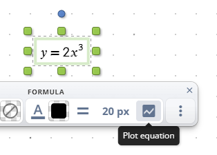
Enter a range in the form of an equation like x ∈ (-6; 2). The graph will be restricted to the specified range. To get the ∈ symbol, enter \in[space] or find the symbol from the equation toolbar.
For example, in polar coordinates, you can limit the angle range to t ∈ (0; π) to plot a semicircle. Similarly, for parameterized equations, you can limit the range of the parameter to get a specific segment of the graph.
If no range is defined, the tool uses default bounds for the variable or parameter based on the graph type. For instance, Cartesian graphs x and y ranges depend on the size of the graph object. Polar graph variable ranges from 0 to 2π and in parameterized equations the default range is t ∈ (-5; 5)
Customizing graph appearance
You can style the graph lines by customizing the equation's appearance:
- Apply a border around the equation to match the graph line style.
- Change the equation's text color to adjust the line color on the graph.
If no border is applied, the text color determines the line color by default.
Supported equation types
The graphing tool supports various types of equations:
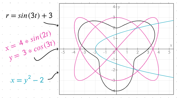
- Cartesian equations: Either
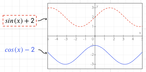
yas a function ofxorxas a function ofy. - Polar equations: Use equations that calculate
ras a function oft,theta, orθ. For example,r = sin(t) + 2. Graphs are plotted over the range[0, 2π]. The equation behaves identically no matter the name of the variable used. - Parameterized equations: Define
xandyas functions of the same parameter on separate lines in the same equation object, for example:x = 4 * sin(2t)y = 3 * cos(3t)
Using variables in equations
You can define variables within equations and reuse them in others. For example: a = x^2, y = 0.2a - 1/a.
The graph updates dynamically whenever the variable or dependent equations are modified.
Supported functions
The graphing tool includes a variety of built-in functions to simplify equation entry and enhance visualization.
Trigonometric functions
- Standard:
sin,cos,tan,csc,sec,cot - Inverse (arc) functions:
arcsin,arccos,arctan - Hyperbolic functions:
sinh,cosh,tanh,csch,sech,coth
Logarithmic functions
log(x): Base 10 logarithmln(x): Natural logarithm (base e)
Other functions
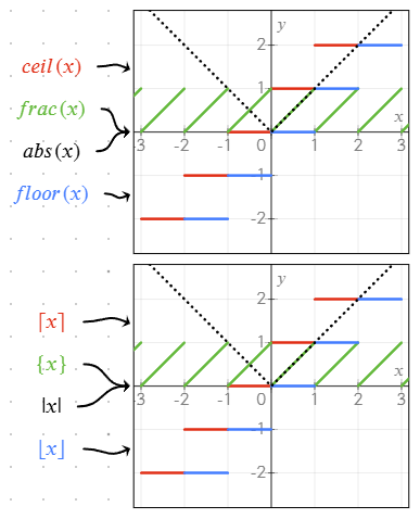
sqrt(x): Square rootabs(x)or|x|: Absolute valuefrac(x)or{x}: Fractional part of a numberfloor(x)or⌊x⌋: Rounds down to the nearest integerceil(x)or⌈x⌉: Rounds up to the nearest integermin(a; b),max(a; b): Minimum/maximum of two or more values
These functions can be combined in equations to create more complex graphs and calculations.
Defining and using custom functions
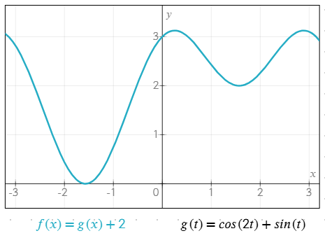
The graphing tool supports defining functions using f(x) = ... notation, making it easy to reuse expressions in multiple equations.
To define a function, use the format: f(x) = cos(2x) + sin(x)
Using functions in equations
Once defined, a function can be referenced in other equations: g(x) = f(x) + 5
If a function is defined with f(x) = ..., it is plotted on the graph. Other variations (e.g., g(t)) are not plotted but can be used in calculations.
Example of multiple functions working together
g(t) = cos(2t) + sin(t)f(x) = g(x) + 2
Custom functions help simplify equations, avoid repetition, and make complex expressions easier to manage.
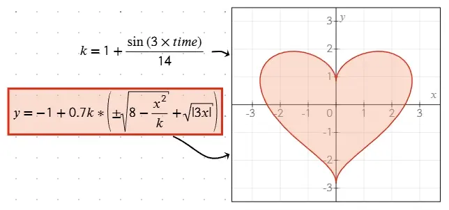
Animating graphs with the 'time' variable
Use the special time variable to create animated graphs. The time variable increments by 1 every second, allowing you to simulate motion or periodic changes in your equations.
For example: r = sin(5 * time) + 2 creates a pulsating circle that updates in real time.
On the image to the right you see a little bit more complex equation utilizing the time variable.
Using predefined variables
The graphing tool includes several predefined constants that can simplify equation creation. These constants are:
piorπ: Mathematical constant π (~3.14159).e: Euler's number (~2.71828).infinityor∞, though it is generally less useful for plotting finite graphs.
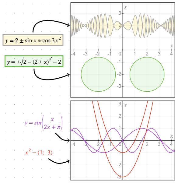
Handling equations with multiple solutions
Using ± for symmetric solutions
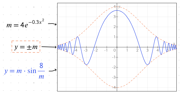
Insert the ± symbol (or +-, which is automatically converted to ±) into the equation to simultaneously plot both the positive and negative results. For example, y = ±sqrt(x) plots both y = sqrt(x) and y = -sqrt(x).
Specifying multiple values
You can specify multiple values or sub-equations in a single equation object by using a list format or multiple lines:
- Bracketed lists: Use
;as a separator inside brackets to define multiple values. For example:y = (1; -1) * xwill plot bothy = xandy = -x. - Separate lines: Press Enter in the equation editor to add multiple sub-equations on different lines. Each line is treated as an independent solution.
These methods allow for flexible creation of graphs with multiple branches or solutions, making it easier to visualize complex relationships.
Troubleshooting equation plotting issues
If an equation is not being drawn, it is likely due to one of the following reasons:
- There is a mistake in the equation syntax (e.g., a missing operator or invalid symbol).
- The range for the variable (e.g.,
xort) is incorrectly defined or not specified. - The equation might be inherently undefined in some regions (e.g., division by zero).
To resolve these issues:
- Double-check your equation for any typos or formatting errors.
- If you’ve specified a range, verify that the interval is valid and relevant to your equation.
- Try retyping the equation to ensure all symbols and operators are properly entered.
If issues persist, test the equation in isolation to confirm its validity.
Performance considerations
When working with complex or dynamic graphs, performance can be impacted. Keep the following tips in mind to maintain a smooth experience:
- Complex equations: Graphs with computationally heavy calculations (e.g., nested trigonometric functions or large ranges) may slow down rendering, especially when combined with animations.
- Rapid oscillations: Equations with high-frequency oscillations (e.g.,
y = tan(1/x)) may be drawn inaccurately near their breaking points due to rendering limitations. To reduce this, limit the range or simplify the equation where possible. - Animation smoothness: If using the
timevariable for animations, ensure your equations do not perform excessive recalculations every frame to maintain smooth motion.
For best results, consider breaking down overly complex graphs into simpler components or using narrower ranges to reduce computation load.
Too many graphs visible on the screen also affects performance negatively. Avoid adding too many graphs near each other for a smoother experience.